Off-policy learning for a turbocharged diesel engine
This is the Numerical Example 2.2 in Chapter 2 of book Robust Adaptive Dynamic Programming by Yu Jiang and Zhong-Ping Jiang
Contents
Parameters configuration
xn = 6;
un = 2;

% Set the weighting matrices for the cost function
Q = diag([100 0 0 0 0 100]);
R = diag([1 1]);

% Initialize the feedback gain matrix
Kinit  = zeros(un,xn);  %Only if A is Hurwitz, K can be set as zero.
K = Kinit;
N  = 100;           %Length of the window, should be at least xn^2+2*xn*un
MaxIteration = 10;  %Max iteration times
T  = 0.01;          %Length of each integration interval

x0 = [20;5;10;2;-1;-2]; %Initial condition

expl_noise_freq = (rand(un,100)-.5)*100; % Exploration noise frequencies

% Matrices to collect online data and perform learning
Dxx=[];
Ixx=[];
Ixu=[];

% Initial condition of the augmented system
X=[x0;kron(x0',x0')';kron(x0,zeros(un,1))]';
Run the simulation and obtain the data matrices \delta_{xx},
%I_{xx}, and I_{xu}

ifLearned = 0;

x_save=[];
t_save=[];

for i=1:N
    % Simulation the system and at the same time collect online info.
    [t,X] = ode45(@(t,x)aug_sys(t,x,K,ifLearned,expl_noise_freq), ...
        [(i-1)*T,i*T],X(end,:));

    %Append new data to the data matrices
    Dxx=[Dxx;kron(X(end,1:xn),X(end,1:xn))-kron(X(1,1:xn),X(1,1:xn))];
    Ixx=[Ixx;X(end,xn+1:xn+xn^2)-X(1,xn+1:xn+xn^2)];
    Ixu=[Ixu;X(end,xn+xn^2+1:end)-X(1,xn+xn^2+1:end)];

    % Keep track of the system trajectories
    x_save=[x_save;X];
    t_save=[t_save;t];
end

ifLearned = 1; % Mark learning finished

P_old = zeros(xn);
P = eye(xn)*10;    % Initialize the previous cost matrix
it = 0;            % Counter for iterations
p_save = [];       % Track the cost matrices in all the iterations
k_save = [];       % Track the feedback gain matrix in each iterations

% The system matrices are copied here only for the purpose of analyzing the
% results
A = [-0.4125    -0.0248        0.0741     0.0089   0          0;
    101.5873    -7.2651        2.7608     2.8068   0          0;
    0.0704       0.0085       -0.0741    -0.0089   0          0.0200;
    0.0878       0.2672        0         -0.3674   0.0044     0.3962;
    -1.8414      0.0990        0          0       -0.0343    -0.0330;
    0            0             0       -359      187.5364   -87.0316];

B = [-0.0042  0.0064
     -1.0360  1.5849
      0.0042  0;
      0.1261  0;
      0      -0.0168;
      0       0];

[Kopt,Popt] = lqr(A,B,Q,R); % Calculate the ideal solution for comparion purpose
k_save  = norm(K-Kopt);  % keep track of the differences between the actual K
% and the idea valu
Off-policy learning using the collected online data
while norm(P-P_old)>1e-8 & it<MaxIteration
    it = it+1;                        % Update and display the # of iters
    P_old = P;                        % Update the previous cost matrix
    QK = Q+K'*R*K;                    % Update the Qk matrix

    Theta = [Dxx,-Ixx*kron(eye(xn),K')-Ixu];  % Left-hand side of
    % the key equation
    Xi = -Ixx*QK(:);                 % Right-hand side of the key equation
    pp = pinv(Theta)*Xi;             % Solve the equations in the LS sense
    P = reshape(pp(1:xn*xn), [xn, xn]);  % Reconstruct the symmetric matrix
    P = (P + P')/2;

    BPv = pp(end-(xn*un-1):end);
    K = inv(R)*reshape(BPv,un,xn)/2;% Get the improved gain matrix
    p_save = [p_save,norm(P-Popt)];   % Keep track of the cost matrix
    k_save = [k_save,norm(K-Kopt)];    % Keep track of the control gains

    disp(['K_', num2str(it), '=']);
    disp(K);
end
K_1=
   47.8326    0.7785    2.9006   42.1547  -24.8884   -0.0909
   38.7653    0.4848    0.5799   20.7823  -11.6976    0.0712

K_2=
   20.3865    0.4444    1.2043   27.3859  -15.6164   -0.1539
   18.1106    0.2602    0.0321   11.4403   -6.2478    0.0293

K_3=
   11.3687    0.3886    0.4585   24.9271  -13.7566   -0.1668
    9.6886    0.2055    0.0395    9.3035   -5.0999    0.0184

K_4=
   10.7552    0.3875    0.4006   24.8447  -13.6680   -0.1672
    9.0006    0.2031    0.0681    9.2034   -5.0791    0.0180

K_5=
   10.7537    0.3875    0.4006   24.8446  -13.6677   -0.1672
    8.9983    0.2031    0.0682    9.2032   -5.0796    0.0180

K_6=
   10.7537    0.3875    0.4006   24.8446  -13.6677   -0.1672
    8.9983    0.2031    0.0682    9.2032   -5.0796    0.0180

K_7=
   10.7537    0.3875    0.4005   24.8446  -13.6677   -0.1672
    8.9983    0.2031    0.0682    9.2032   -5.0796    0.0180

K_8=
   10.7537    0.3875    0.4005   24.8446  -13.6677   -0.1672
    8.9983    0.2031    0.0682    9.2032   -5.0796    0.0180

K_9=
   10.7537    0.3875    0.4005   24.8446  -13.6677   -0.1672
    8.9983    0.2031    0.0682    9.2032   -5.0796    0.0180

K_10=
   10.7537    0.3875    0.4006   24.8446  -13.6677   -0.1672
    8.9983    0.2031    0.0682    9.2032   -5.0796    0.0180
Post-learning simulations
[tt,xx]=ode45(@(t,x)aug_sys(t,x,K,ifLearned,expl_noise_freq), ...
    [t(end) 10],X(end,:)');

% Keep track of the post-learning trajectories
t_final = [t_save;tt];
x_final = [x_save;xx];

% For comparson, also get the unlearned simulation
[ttt,xxx]=ode45(@(t,x)aug_sys(t,x,Kinit,ifLearned,expl_noise_freq), ...
    [t(end) 10],X(end,:)');
t_unlearned = [t_save;ttt];
x_unlearned = [x_save;xxx];
Plotting results
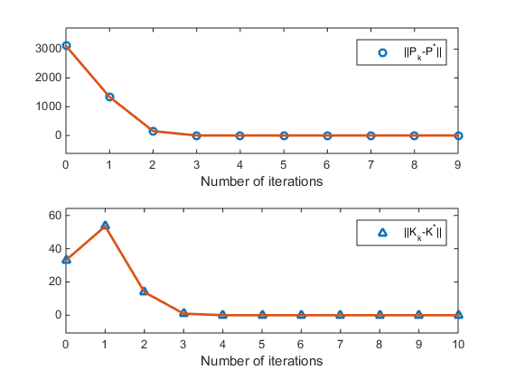
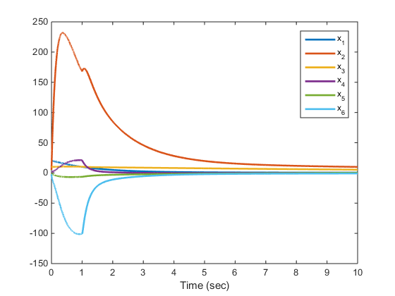
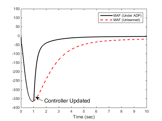
figure(1)
subplot(211)
plot(0:length(p_save)-1,p_save,'o',0:length(p_save)-1,p_save,'Linewidth',2);
ylim([-max(p_save)*0.2 max(p_save)*1.2]);
legend('||P_k-P^*||')
xlabel('Number of iterations')

subplot(212)
plot(0:length(k_save)-1,k_save,'^',0:length(k_save)-1,k_save,'Linewidth',2)
ylim([-max(k_save)*0.2 max(k_save)*1.2]);
legend('||K_k-K^*||')
xlabel('Number of iterations')

% Uncomment to save figure
% print('Ch2_ex2_fig1_pk','-depsc')

figure(2)
plot(t_final,x_final(:,1:6),'Linewidth',2)
legend('x_1','x_2','x_3','x_4','x_5','x_6')
xlabel('Time (sec)')

figure(3)
plot(t_final, 3.6*x_final(:,6),'k-', ...
     ttt, 3.6*xxx(:,6),'r--', ...
    'Linewidth',2)
ylim([-400 150])

legend('MAF (Under ADP)', 'MAF (Unlearned)')
xlabel('Time (sec)','FontSize',12)

% Create textarrow
annotation(figure(3),'textarrow',[0.2630173564753 0.218958611481976],...
	[0.166023166023166 0.198841698841699],'String',{'Controller Updated'},...
	'FontSize',14);

% Uncomment to save figure
% print('Ch2_ex2_fig2_y','-depsc')
Display results
disp('Approximate Cost Matrix')
P
disp('Optimal Cost Matrix')
Popt
disp('Approximate Gain Matrix')
K
disp('Optimal Gain Matrix')
Kopt
Approximate Cost Matrix

P =

  766.7586    1.4019   97.3262  119.0937 -111.2552    0.6265
    1.4019    0.1032   -0.6581    3.9893   -1.8221    0.0150
   97.3262   -0.6581   71.6942   -1.3764  -29.0644    0.0230
  119.0937    3.9893   -1.3764  233.8101 -126.0950   -1.1828
 -111.2552   -1.8221  -29.0644 -126.0950   88.0805    0.5859
    0.6265    0.0150    0.0230   -1.1828    0.5859    0.5687

Optimal Cost Matrix

Popt =

  766.7586    1.4020   97.3265  119.0937 -111.2549    0.6265
    1.4020    0.1032   -0.6581    3.9893   -1.8221    0.0150
   97.3265   -0.6581   71.6915   -1.3767  -29.0678    0.0230
  119.0937    3.9893   -1.3767  233.8101 -126.0952   -1.1828
 -111.2549   -1.8221  -29.0678 -126.0952   88.0775    0.5859
    0.6265    0.0150    0.0230   -1.1828    0.5859    0.5687

Approximate Gain Matrix

K =

   10.7537    0.3875    0.4006   24.8446  -13.6677   -0.1672
    8.9983    0.2031    0.0682    9.2032   -5.0796    0.0180

Optimal Gain Matrix

Kopt =

   10.7537    0.3875    0.4006   24.8446  -13.6677   -0.1672
    8.9983    0.2031    0.0681    9.2032   -5.0796    0.0180