Ch4Ex2_main

GADP for a scalar polynomial system
Setting parameters
Start online simulation
Post-process and plot results
LocalPostProcess: Process results and generate figures
LocalOnlinePI
LocalComputeObjective
LocalComputeControlSignal

function SimResults = Ch4Ex2_main()

GADP for a scalar polynomial system

Demo #1 for Global Adaptive Dynamic Programming for Continuous-time Nonlinear Systems, by Yu Jiang and Zhong-Ping Jiang, IEEE Transasctions on Automatic Control, 2015

This paper can be found at 1. http://ieeexplore.ieee.org/xpl/articleDetails.jsp?arnumber=7063901 2. http://arxiv.org/pdf/1401.0020.pdf

System requirements: - MATLAB (Manually Tested in MATLAB R2014b) - MATLAB Symbolic Toolbox - CVX (free to download at http://cvxr.com/cvx/)

Contact: yu.jiang@nyu.edu (Yu Jiang)

Setting parameters

Parameters for Simulation the dynamic system

SysParams.Q = 0.01*[1 0 0;0 1 0;0 0 0];  % The cost function will be
                                         % ([x]_{1,3})'*Q*[x]_{1,3}+u^2
SysParams.noiseFlag = true;   % Inicator for noise on/off
SysParams.K = [0.1 0 0.01];   % Initial feeback gain matrix
SysParams.F = [0 0.01 0];     % System dynamics dx = F*[x]_1,3 + u,
                              % F is not used in Online Policy Iteration
SysParamsInit = SysParams;    % Make a copy of initial parameters

% Parameters for learning
Params.iter_tol = 0.007;
Params.T = 0.1;          % Length of each time interval for data collection
Params.MaxIter = 10;     % Maximum iteration numbers
Params.IterInterval = 5; % Length of each time interval for learning
Params.xinit = 2;        % Initial condition for the actual state x


% Other params
x = [Params.xinit;zeros(9,1)]'; % Initial condition for the augmented x
P = eye(2)*10;                % Initialize V_0: ([x]_{1,2})'*P*[x]_{1,2}
Pold = -100*eye(2);           % Initialize V_{-1}

% Simulation results to export
SimResults.Ksave = SysParams.K;  % Keep track of the feedback gains
SimResults.Psave = P(:)';        % Keep track of the value function
SimResults.Usave = [];           % Actual control signal during simulation
SimResults.Xsave=[];             % Actual x(t) during simulation
SimResults.Tsave=[];             % Sample time points during simulation


% caculate the weights for V
c = LocalComputeObjective(-1, 1);

Start online simulation

for i = 0:Params.MaxIter-1
   % Data collection
   Theta = [];Sigma = []; Xi = [];  % Data matrices for online learning
    for j = 0:Params.IterInterval/Params.T-1
        [t,x] = ode45(@(t,x) SystemWrapper(t,x,SysParams), ...
            [j,j+1]*Params.T + i*Params.IterInterval, ...
            [x(end,1) zeros(1,9)]);
        Theta = [Theta;
                (x(end,1)^2-x(1,1)^2) (x(end,1)^3-x(1,1)^3) (x(end,1)^4-x(1,1)^4)];
        Sigma = [Sigma;
                 x(end,2:6)  -x(end,7:9)];
        Xi = [Xi; x(end,10)];
        SimResults.Tsave = [SimResults.Tsave;t];
        SimResults.Xsave = [SimResults.Xsave;x(:,1)];
        for k=1:length(t)
            SimResults.Usave = [SimResults.Usave;
               LocalComputeControlSignal(x(k,1),SysParams.K,...
               SysParams.noiseFlag,t(k))];
        end
    end

    % SOS-based Online Policy iteration
    if norm(P(:)-Pold(:)) > Params.iter_tol
        % Calling local function for policy improvement and policy
        % evaluation. Notice that we do not pass in the systen dynamics,
        % i.e, the F vector. Because online learning does not rely on it.
        [Pn,K] = LocalOnlinePI(Sigma,Xi,Theta,... % Data matrices collected online
                               c,  ... % weights
                               P);     % previous value function
        Pold = P; P = Pn; % Save the current and the old P
        SysParams.noiseFlag = true;
        SysParams.K = K;
        SimResults.Ksave = [SimResults.Ksave; K(:)'];
        SimResults.Psave = [SimResults.Psave; P(:)'];
        % Qlave=[Qlave;dQl(:)'];

    else
        SysParams.noiseFlag = false;
        disp('Convergence has been attained ...update is not necessary')
    end
end

Post-process and plot results

SimResults.hFigs = LocalPostProcess(SysParams, SysParamsInit, ...
   SimResults,Params, P);

end

LocalPostProcess: Process results and generate figures

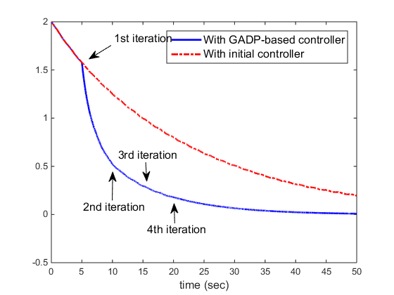
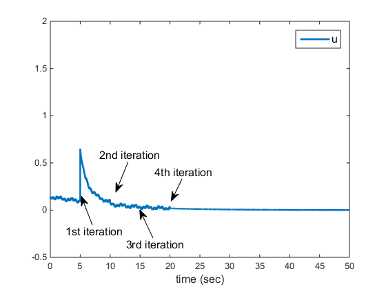
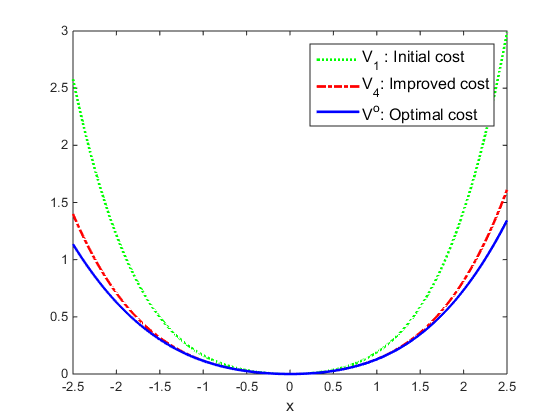
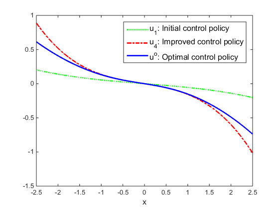
function hFigs = LocalPostProcess(SysParams, SysParamsInit,SimResults, Params, P)
% Figure 1:
% Comparison of x between GADP and unlearned system
hFig1 = figure(1);
[t0,y0] = ode45(@(t,x) SystemWrapper(t,x,SysParamsInit),...
    [0 50], ...
    [Params.xinit, zeros(1,9)]);
y0 = y0(:,1); % Only need the first column for the actual x
for i=1:length(t0)
 u0(i) = SysParamsInit.K * y0(i).^[1 2 3]'; % Unleared controller
end

plot(SimResults.Tsave, SimResults.Xsave, 'b-', ...  % Learned
     t0,y0, 'r-.', ...                              % Unlearned
     'linewidth', 2)
axis([0 50 -.5 2])
myLegend = legend('With GADP-based controller', 'With initial controller');
set(myLegend, 'Fontsize', 12);
xlabel('time (sec)', 'FontSize', 12)
%ylabel('x', 'FontSize', 12)

% Create textarrows
annotation(hFig1,'textarrow', ...
    [0.281132075471698 0.226415094339623],...
    [0.845386533665835 0.800498753117207],'TextEdgeColor','none',...
    'FontSize',12,...
    'String',{'1st iteration'});
annotation(hFig1,'textarrow',...
    [0.443396226415094 0.44188679245283],...
    [0.244389027431421 0.309127182044887],'TextEdgeColor','none',...
    'FontSize',12,...
    'String',{'4th iteration'});
annotation(hFig1,'textarrow',...
    [0.369811320754717 0.372452830188679],...
    [0.448877805486284 0.386334164588527],'TextEdgeColor','none',...
    'FontSize',12,...
    'String',{'3rd iteration'});
annotation(hFig1,'textarrow',...
    [0.284905660377358 0.286037735849057],...
    [0.321695760598504 0.416408977556109],'TextEdgeColor','none', ...
    'FontSize',12,...
    'String',{'2nd iteration'});

% Figure 2
hFig2 = figure(2);
plot(SimResults.Tsave, SimResults.Usave,'Linewidth',2)
myLegend = legend('u');
set(myLegend, 'FontSize', 12);
xlabel('time (sec)', 'FontSize', 12)
axis([0 50 -0.5 2]);
% Create textarrows
annotation(hFig2 ,'textarrow',[0.239092495636998 0.2107082880569],...
    [0.221748400852878 0.320754616656652],'TextEdgeColor','none', ...
    'FontSize',12,...
    'String',{'1st iteration'});
annotation(hFig2 ,'textarrow',[0.396160558464223 0.361981626000198],...
    [0.176972281449893 0.27332776800004],'TextEdgeColor','none', ...
    'FontSize',12,...
    'String',{'3rd iteration'});
annotation(hFig2 ,'textarrow',[0.331588132635253 0.2999993414337],...
    [0.439232409381663 0.335385523398326],'TextEdgeColor','none', ...
    'FontSize',12,...
    'String',{'2nd iteration'});
annotation(hFig2 ,'textarrow',[0.471204188481675 0.443631993150911],...
    [0.37953091684435 0.304862789720793],'TextEdgeColor','none', ...
    'FontSize',12,...
    'String',{'4th iteration'});



% Figures 3:
% Comparing the initial, the improved, and the ideal value fcn
syms v(y)
F = SysParams.F;
% Solve the HJB analytically
vsx = dsolve(diff(v)*(F(1)*y+F(2)*y^2+F(3)*y^3) + 0.01*(y^2+y^4)-1/4*(diff(v))^2==0, v(0)==0);
vsx = vsx(1);
x = -2.5:.01:2.5;
vn = []; % V_n
v1 = []; % V_1
vs = []; % Optimal V*
us = []; % Optimal u*
u1 = []; % Initial u_1
un = []; % Improved u_n
P1 = [SimResults.Psave(2,1) SimResults.Psave(2,2);
      SimResults.Psave(2,3) SimResults.Psave(2,4)] ;

for y = x
vn = [vn [y y^2]*P*[y ;y^2]];
v1 = [v1 [y y^2]*P1*[y ;y^2]];
vs = [vs eval(vsx)];
u1 = [u1 -1/2*SysParamsInit.K*[y;y^2;y^3]];
un = [un -1/2*SysParams.K'*[y;y^2;y^3]];
us = [us -1/2*eval(diff(vsx))];
%(y*(y*(101*y^2 + 100)^(1/2) + 101*y^2 + 100))/(50*(101*y^2 + 100)^(1/2))
end

hFig3 = figure(3);
plot(x,v1,'g:',x,vn,'r-.',x,vs,'b','linewidth',2)
myLegend = legend('V_1 : Initial cost', 'V_4: Improved cost', ...
    'V^o: Optimal cost');
set(myLegend, 'FontSize', 12);
xlabel('x', 'FontSize', 12)

% Figures 4:
% Comparing the initial, the improved, and the ideal control input
hFig4 = figure(4);
plot(x,u1,'g:',x,un,'r-.',x,us,'b','linewidth',2)
myLegend = legend('u_1: Initial control policy', ...
    'u_4: Improved control policy', ...
    'u^o: Optimal control policy');
set(myLegend, 'FontSize', 12);
xlabel('x', 'FontSize', 12)

% Export all figure handles
hFigs = [hFig1; hFig2; hFig3; hFig4];

end

ans = 

    Ksave: [4x3 double]
    Psave: [4x4 double]
    Usave: [22612x1 double]
    Xsave: [22612x1 double]
    Tsave: [22612x1 double]
    hFigs: [4x1 Figure]

LocalOnlinePI

Local function to implement the online ADP method. Note1: CVX solver is required (Download: http://cvxr.com/cvx/) Note2: The learning process does not depend on the system dynamics (F)

function [Pn,K] = LocalOnlinePI(Sigma,Xi,Theta,c,P)
cvx_begin sdp
variable pv(3,1)
variable dQl(3,3) symmetric
% SDP Objective function
minimize(c(1)*pv(1)+c(3)*pv(3))
% 1) Equality constraint
LnK = -inv(Sigma'*Sigma)*Sigma'*(Xi + Theta*pv(:));
% 2) SOS constraint:
%    L*[x]_2,6 is SOS
% i.e., there exists Ql>0, such that
%    L*[x]_2,6 = ([x]_1,3)'*Ql*[x]_1,3
LnK(1) == dQl(1,1);                        %#ok<*EQEFF> CVX Syntax
LnK(2) == dQl(1,2) + dQl(2,1);
LnK(3) == dQl(1,3) + dQl(3,1) + dQl(2,2);
LnK(4) == dQl(3,2) + dQl(2,3);
LnK(5) == dQl(3,3);
dQl >= 0;                                  %#ok<*VUNUS> CVX Syntax
% 3) SOS constraint
%    pv_old*[x]_1,3 - pv*[x]_1,3 is SOS
% This implies that
% V_old >= V_new (i.e.,the value function is reduced)
Pn = [ pv(1) 1/2*(pv(2)); 1/2*(pv(2)) pv(3)];
Pn <= P;
K = LnK(6:8);
cvx_end
end

 
Calling SDPT3 4.0: 9 variables, 5 equality constraints
------------------------------------------------------------

 num. of constraints =  5
 dim. of sdp    var  =  3,   num. of sdp  blk  =  1
 dim. of socp   var  =  3,   num. of socp blk  =  1
*******************************************************************
   SDPT3: Infeasible path-following algorithms
*******************************************************************
 version  predcorr  gam  expon  scale_data
   HKM      1      0.000   1        0    
it pstep dstep pinfeas dinfeas  gap      prim-obj      dual-obj    cputime
-------------------------------------------------------------------
 0|0.000|0.000|1.7e+00|3.2e+01|1.5e+04|-1.265389e+01  0.000000e+00| 0:0:00| chol  1  1 
 1|0.914|0.994|1.5e-01|4.5e-01|1.3e+03|-9.247077e+00 -1.875106e+02| 0:0:01| chol  1  1 
 2|0.798|0.832|3.0e-02|9.8e-02|3.0e+02|-3.546474e+01 -3.842428e+01| 0:0:01| chol  1  1 
 3|0.983|0.989|5.0e-04|9.9e-03|2.1e+01|-9.207216e+00 -2.525519e+01| 0:0:01| chol  1  1 
 4|1.000|0.939|6.1e-07|9.8e-04|1.3e+00|-9.419454e+00 -1.074777e+01| 0:0:01| chol  1  1 
 5|0.932|1.000|4.2e-08|2.9e-05|9.8e-02|-1.050540e+01 -1.060299e+01| 0:0:01| chol  2  2 
 6|0.884|0.981|1.7e-08|3.4e-06|9.3e-03|-1.055724e+01 -1.056651e+01| 0:0:01| chol  2  2 
 7|0.966|0.976|5.4e-08|3.6e-07|4.2e-04|-1.056243e+01 -1.056283e+01| 0:0:01| chol  2  2 
 8|0.953|0.982|3.3e-09|1.1e-08|1.7e-05|-1.056268e+01 -1.056270e+01| 0:0:01| chol  2  2 
 9|0.968|1.000|7.1e-11|6.6e-10|1.3e-06|-1.056270e+01 -1.056270e+01| 0:0:01| chol  3  3 
10|1.000|1.000|1.2e-10|1.4e-11|1.2e-07|-1.056270e+01 -1.056270e+01| 0:0:01|
  stop: max(relative gap, infeasibilities) < 1.49e-08
-------------------------------------------------------------------
 number of iterations   = 10
 primal objective value = -1.05626961e+01
 dual   objective value = -1.05626963e+01
 gap := trace(XZ)       = 1.18e-07
 relative gap           = 5.36e-09
 actual relative gap    = 8.71e-09
 rel. primal infeas     = 1.20e-10
 rel. dual   infeas     = 1.43e-11
 norm(X), norm(y), norm(Z) = 9.9e+00, 6.4e+00, 6.5e+00
 norm(A), norm(b), norm(C) = 7.5e+01, 5.2e+02, 2.1e+00
 Total CPU time (secs)  = 0.65  
 CPU time per iteration = 0.06  
 termination code       =  0
 DIMACS: 1.4e-10  0.0e+00  1.5e-11  0.0e+00  8.7e-09  5.4e-09
-------------------------------------------------------------------
------------------------------------------------------------
Status: Solved
Optimal value (cvx_optval): +0.103971
 
 
Calling SDPT3 4.0: 9 variables, 4 equality constraints
   For improved efficiency, SDPT3 is solving the dual problem.
------------------------------------------------------------

 num. of constraints =  4
 dim. of sdp    var  =  3,   num. of sdp  blk  =  1
 dim. of socp   var  =  3,   num. of socp blk  =  1
*******************************************************************
   SDPT3: Infeasible path-following algorithms
*******************************************************************
 version  predcorr  gam  expon  scale_data
   HKM      1      0.000   1        0    
it pstep dstep pinfeas dinfeas  gap      prim-obj      dual-obj    cputime
-------------------------------------------------------------------
 0|0.000|0.000|5.7e+00|1.7e+01|3.1e+02| 1.617063e-01  0.000000e+00| 0:0:00| chol  1  1 
 1|1.000|0.569|3.0e-06|7.5e+00|1.6e+02| 3.447710e-01  3.727454e+00| 0:0:00| chol  1  1 
 2|1.000|0.988|3.1e-06|9.9e-02|2.5e+00| 3.423958e-01  5.715867e-02| 0:0:00| chol  1  1 
 3|1.000|1.000|8.5e-07|1.0e-03|2.5e-01| 2.477562e-01  9.856892e-03| 0:0:00| chol  1  1 
 4|0.880|1.000|1.1e-07|1.0e-04|3.0e-02| 4.033566e-02  1.098353e-02| 0:0:00| chol  1  1 
 5|1.000|0.883|1.7e-09|2.1e-05|9.4e-03| 3.041046e-02  2.103547e-02| 0:0:00| chol  1  1 
 6|0.979|0.937|5.8e-10|2.2e-06|7.3e-04| 2.459428e-02  2.387157e-02| 0:0:00| chol  1  1 
 7|0.969|0.982|7.0e-11|1.4e-07|2.1e-05| 2.409139e-02  2.407090e-02| 0:0:00| chol  1  1 
 8|0.951|0.971|1.8e-11|4.0e-09|9.2e-07| 2.407706e-02  2.407615e-02| 0:0:00| chol  1  1 
 9|1.000|1.000|3.1e-12|3.7e-12|1.2e-07| 2.407654e-02  2.407642e-02| 0:0:00| chol  1  1 
10|0.996|0.997|1.3e-14|1.0e-12|1.5e-09| 2.407648e-02  2.407647e-02| 0:0:00|
  stop: max(relative gap, infeasibilities) < 1.49e-08
-------------------------------------------------------------------
 number of iterations   = 10
 primal objective value =  2.40764756e-02
 dual   objective value =  2.40764741e-02
 gap := trace(XZ)       = 1.54e-09
 relative gap           = 1.47e-09
 actual relative gap    = 1.47e-09
 rel. primal infeas     = 1.28e-14
 rel. dual   infeas     = 1.01e-12
 norm(X), norm(y), norm(Z) = 2.4e+00, 3.2e-02, 4.6e-02
 norm(A), norm(b), norm(C) = 4.2e+00, 1.8e+00, 1.0e+00
 Total CPU time (secs)  = 0.12  
 CPU time per iteration = 0.01  
 termination code       =  0
 DIMACS: 1.4e-14  0.0e+00  1.0e-12  0.0e+00  1.5e-09  1.5e-09
-------------------------------------------------------------------
------------------------------------------------------------
Status: Solved
Optimal value (cvx_optval): +0.0798941
 
 
Calling SDPT3 4.0: 9 variables, 4 equality constraints
   For improved efficiency, SDPT3 is solving the dual problem.
------------------------------------------------------------

 num. of constraints =  4
 dim. of sdp    var  =  3,   num. of sdp  blk  =  1
 dim. of socp   var  =  3,   num. of socp blk  =  1
*******************************************************************
   SDPT3: Infeasible path-following algorithms
*******************************************************************
 version  predcorr  gam  expon  scale_data
   HKM      1      0.000   1        0    
it pstep dstep pinfeas dinfeas  gap      prim-obj      dual-obj    cputime
-------------------------------------------------------------------
 0|0.000|0.000|5.6e+00|1.8e+01|3.1e+02| 3.773139e-02  0.000000e+00| 0:0:00| chol  1  1 
 1|1.000|0.692|2.0e-06|5.5e+00|1.0e+02| 5.918167e-02  3.074580e+00| 0:0:00| chol  1  1 
 2|1.000|0.988|2.2e-06|7.3e-02|1.4e+00| 5.887067e-02  4.147024e-02| 0:0:00| chol  1  1 
 3|1.000|1.000|6.9e-07|1.0e-03|6.5e-02| 5.010300e-02  1.803558e-03| 0:0:00| chol  1  1 
 4|0.877|1.000|1.3e-07|1.0e-04|8.2e-03| 9.296373e-03  1.716321e-03| 0:0:00| chol  1  1 
 5|0.780|1.000|2.9e-08|1.0e-05|2.1e-03| 4.791892e-03  2.700389e-03| 0:0:00| chol  1  1 
 6|0.679|0.944|9.2e-09|1.5e-06|8.2e-04| 4.345632e-03  3.529860e-03| 0:0:00| chol  1  1 
 7|0.898|1.000|9.4e-10|1.0e-07|9.3e-05| 3.765499e-03  3.672890e-03| 0:0:00| chol  1  1 
 8|0.941|0.988|6.8e-11|1.4e-09|4.2e-06| 3.708477e-03  3.704241e-03| 0:0:00| chol  1  1 
 9|0.994|1.000|3.9e-12|1.4e-11|2.3e-07| 3.705355e-03  3.705130e-03| 0:0:00| chol  1  1 
10|0.994|0.997|2.4e-14|1.0e-12|2.7e-09| 3.705234e-03  3.705232e-03| 0:0:00|
  stop: max(relative gap, infeasibilities) < 1.49e-08
-------------------------------------------------------------------
 number of iterations   = 10
 primal objective value =  3.70523444e-03
 dual   objective value =  3.70523172e-03
 gap := trace(XZ)       = 2.72e-09
 relative gap           = 2.70e-09
 actual relative gap    = 2.70e-09
 rel. primal infeas     = 2.45e-14
 rel. dual   infeas     = 1.04e-12
 norm(X), norm(y), norm(Z) = 3.2e+00, 6.2e-03, 9.1e-03
 norm(A), norm(b), norm(C) = 4.2e+00, 1.8e+00, 1.0e+00
 Total CPU time (secs)  = 0.11  
 CPU time per iteration = 0.01  
 termination code       =  0
 DIMACS: 2.6e-14  0.0e+00  1.0e-12  0.0e+00  2.7e-09  2.7e-09
-------------------------------------------------------------------
------------------------------------------------------------
Status: Solved
Optimal value (cvx_optval): +0.0761889
 
Convergence has been attained ...update is not necessary
Convergence has been attained ...update is not necessary
Convergence has been attained ...update is not necessary
Convergence has been attained ...update is not necessary
Convergence has been attained ...update is not necessary
Convergence has been attained ...update is not necessary
Convergence has been attained ...update is not necessary

LocalComputeObjective

Compute the objective function for the SOSp in Policy Iterations. The objective depends on the interval [x_min, x_max]. This requires MATLAB Symbolic Toolbox.

function c = LocalComputeObjective(x_min, x_max)
syms z
c = double(int(z.^[2,3,4], x_min,x_max));
end

LocalComputeControlSignal

Compute the control input

function u = LocalComputeControlSignal(x,K,noiseFlag,t)
 u = -1/2*K(:)'*x.^[1 2 3]'+ ExplorationNoise(t)*noiseFlag;
 u = abs(u);
end

Contents