Contents
function Ch6Ex1_main()
RADP for a ten-machine power system
This is the Matlab code used for the paper:
Yu Jiang and Zhong-Ping Jiang, "Robust Adaptive Dynamic Programming for Large-Scale Systems with an Application to Multimachine Power Systems," IEEE Transactions on Circuits and Systems II: Params.Express Briefs, vol. 59, no. 10, pp. 693-697, 2012.
The code is free for everyone to use. Please cite the above paper in your publication if you do use the code.
Please contact yu.jiang@nyu.edu if you find any bugs or have any suggestions on improving the code. Thanks!
%load the parameters
Params = Local_load_params();
[Nm, pm, imxx, imuu] = deal(Params.Nm, Params.pm, Params.imxx, Params.imuu);

% simulate the system until 4s
% operating in steady-state from 0s to 1s
% Kadp = zeros(1,3,Nm); % Preallocating.
Kadp = repmat([10 50 0],[1,1,Nm-1]);
disp('Simulating the system on steady state to 1s...')
[t0,y0] = ode45(@(t,x) Local_mmsys_online_radp(t,x,Kadp),[0,1],zeros(15*(Nm-1),1));

% add an impulse disturbance at 1s
disp('Adding an impulse disturbance at 1s and simulating to 4s...')
[t1,y1]=ode45(@(t,x) Local_mmsys_online_radp(t,x,Kadp), ...
    [1,4],y0(end,:)'-[kron(pm(2:end),[0,0,1]),zeros(1,12*(Nm-1))]');

y = y1(end,:);
N = 20;           % # of learning intervals
stop_tol = 0.01;  % Stop criterion

Ixx = zeros(N,9,Nm-1);
Ixu = zeros(N,3,Nm-1);
Dxx = zeros(N,6,Nm-1);

yy = [y0;y1];
tt = [t0;t1];

% Simulate the system from 4s to 5s to collect enough online information
% for later offpolicy learning
for cti = 0:N-1
    disp(['simulating the ', num2str(cti+1),'-th interval...', ...
        num2str(N-cti), 'left']);
    % simulate the trajectories for learning
    [t,y]=ode45(@(t,x) Local_mmsys_online_radp(t,x,Kadp),[4+cti/N,4+(cti+1)/N],y(end,:));
    for ctj = 1:Nm-1
        Ixx(cti+1,:,ctj) = y(end,imxx(ctj):imxx(ctj)+8)-y(1,imxx(ctj):imxx(ctj)+8);
        Ixu(cti+1,:,ctj) = y(end,imuu(ctj):imuu(ctj)+2)-y(1,imuu(ctj):imuu(ctj)+2);
        Dxx(cti+1,:,ctj) = [y(end,1+(ctj-1)*3)^2-y(1,1+(ctj-1)*3)^2
            y(end,1+(ctj-1)*3)*y(end,2+(ctj-1)*3)-y(1,1+(ctj-1)*3)*y(1,2+(ctj-1)*3)
            y(end,1+(ctj-1)*3)*y(end,3+(ctj-1)*3)-y(1,1+(ctj-1)*3)*y(1,3+(ctj-1)*3)
            y(end,2+(ctj-1)*3)^2-y(1,2+(ctj-1)*3)^2
            y(end,2+(ctj-1)*3)*y(end,3+(ctj-1)*3)-y(1,2+(ctj-1)*3)*y(1,3+(ctj-1)*3)
            y(end,3+(ctj-1)*3)^2-y(1,3+(ctj-1)*3)^2]';
    end
    yy = [yy;y];
    tt = [tt;t];
end

% off-Policy learning for all Generators

K = repmat([10 50 0],[1,1,Nm-1]);

for ctj = 1:Nm-1
    Kprev = [100 100 100];
    it=0;
    while (norm(K(:,:,ctj)-Kprev)>stop_tol)
        it = it+1;
        Kprev = K(:,:,ctj);
        Qk = 1000*eye(3)+K(:,:,ctj)'*K(:,:,ctj);
        Theta = [Dxx(:,:,ctj) -2*Ixx(:,:,ctj)*kron(eye(3),K(:,:,ctj)')-2*Ixu(:,:,ctj)*kron(eye(3),1)];
        Psi = -Ixx(:,:,ctj)*Qk(:);
        % pv=inv(Theta'*Theta)*Theta'*Psi;
        pv = pinv(Theta)*Psi;
        K(:,:,ctj)=pv(end-2:end)';
    end
    Kadp(:,:,ctj) = K(:,:,ctj);
    disp(['The' num2str(ctj+1) '-th machine stopped learning after' num2str(it) 'iterations'])
end
Simulate the post-learning performance
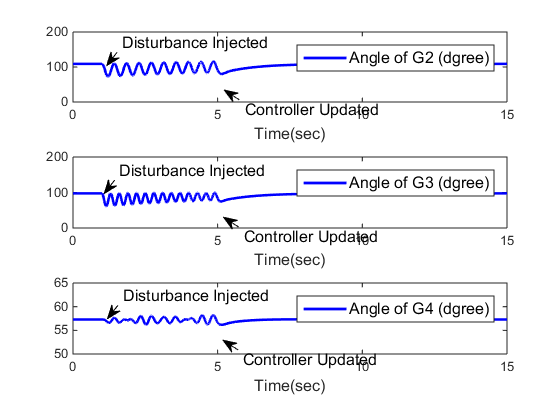
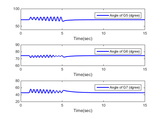
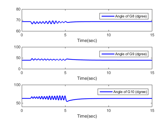
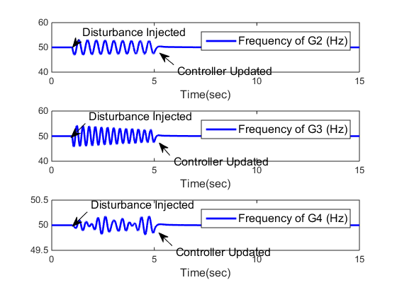
[t,y]=ode45(@(t,x) Local_mmsys_online_radp(t,x,Kadp),[5,15],y(end,:));
y=[yy;y];t=[tt;t];

% Clean up
clear Local_mmsys_online_radp

% plot the angles
Local_plot(t,y,Params.dlt0);
end
Local_mmsys_online_radp
Local function to simulat the dynamics of the multimachine power system.
function dxx = Local_mmsys_online_radp(t,xx, Kadp)

persistent Params

if isempty(Params)
    Params = Local_load_params();
end

A = Params.A;
B = Params.B;
Nm = Params.Nm;

x = zeros(3,Nm);
for ct = 2:Nm
    id = (ct-2)*3 + 1:(ct-2)*3+3;
    x(:,ct) = xx(id);
end

% calculate angular differences in matrix form
dlt=zeros(Nm);d=zeros(1,Nm);
for i=1:Nm
    dlt(i,:)=x(1,i)+Params.dlt0(i)-x(1,:)-Params.dlt0';
    d(i)= Params.E(i)*(Params.E.*(x(2,i)-x(2,:)))*(Params.BX(i,:).*cos(dlt(i,:))-Params.GX(i,:).*sin(dlt(i,:)))';
end
u = zeros(Nm,1);
for i=2:Nm
    if t>=4 && t<=5 % learning stage is between 4s and 5s
        u(i) = -Kadp(:,:,i-1)*x(:,i)+0.001*sin(100*t);
    else
        u(i) = -Kadp(:,:,i-1)*x(:,i);
    end
end

for i = 2:Nm
    dx(:,i-1) = A(:,:,i)*x(:,i)+B(:,:,i)*(u(i)-d(i));
end

dIxxu=zeros(12,Nm-1);
if t>=4 && t<=5
    for i=2:Nm
        dIxxu(:,i-1)=[kron(x(:,i),x(:,i));kron(x(:,i),u(i)-d(i))];
    end
end
dxx = [dx(:);
    dIxxu(:)];
end
Adding an impulse disturbance at 1s and simulating to 4s...
simulating the 1-th interval...20left
simulating the 2-th interval...19left
simulating the 3-th interval...18left
simulating the 4-th interval...17left
simulating the 5-th interval...16left
simulating the 6-th interval...15left
simulating the 7-th interval...14left
simulating the 8-th interval...13left
simulating the 9-th interval...12left
simulating the 10-th interval...11left
simulating the 11-th interval...10left
simulating the 12-th interval...9left
simulating the 13-th interval...8left
simulating the 14-th interval...7left
simulating the 15-th interval...6left
simulating the 16-th interval...5left
simulating the 17-th interval...4left
simulating the 18-th interval...3left
simulating the 19-th interval...2left
simulating the 20-th interval...1left
The2-th machine stopped learning after13iterations
The3-th machine stopped learning after11iterations
The4-th machine stopped learning after11iterations
The5-th machine stopped learning after11iterations
The6-th machine stopped learning after10iterations
The7-th machine stopped learning after10iterations
The8-th machine stopped learning after11iterations
The9-th machine stopped learning after11iterations
The10-th machine stopped learning after10iterations
Local_plot
Plot results
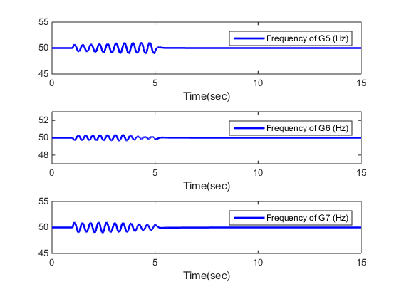
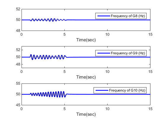
function Local_plot(t,y,dlt0)
%Plot the power angles of G2-G10
figure(1)
subplot(311)
plot(t,(y(:,1)+dlt0(2))*180/pi,'b','linewidth',2)
xlabel('Time(sec)', 'FontSize', 12)
l = legend('Angle of G2 (dgree)');
set(l, 'FontSize', 12)
axis([0 15 0 200])
subplot(312)
plot(t,(y(:,4)+dlt0(3))*180/pi,'b','linewidth',2)
xlabel('Time(sec)', 'FontSize', 12)
l = legend('Angle of G3 (dgree)');
set(l, 'FontSize', 12)
axis([0 15 0 200])
subplot(313)
plot(t,(y(:,7)+dlt0(4))*180/pi,'b','linewidth',2)
xlabel('Time(sec)', 'FontSize', 12)
l = legend('Angle of G4 (dgree)');
set(l, 'FontSize', 12)
axis([0 15 50 65])
annotation(figure(1),'textarrow',[0.424517593643587 0.398365782488103],...
	[0.16729088639201 0.189882327941137],'String',{'Controller Updated'},...
	'FontSize',12);
annotation(figure(1),'textarrow',[0.425440032308299 0.399288221152816],...
	[0.460015659616231 0.482607101165358],'String',{'Controller Updated'},...
	'FontSize',12);
annotation(figure(1),'textarrow',[0.426787741203178 0.400635930047695],...
	[0.762796504369538 0.785387945918666],'String',{'Controller Updated'},...
	'FontSize',12);
annotation(figure(1),'textarrow',[0.208516886930984 0.190650614335506],...
	[0.874592833876222 0.84401986774277],'String',{'Disturbance Injected'},...
	'FontSize',12);
annotation(figure(1),'textarrow',[0.204111600587371 0.186245327991894],...
	[0.570032573289903 0.539459607156451],'String',{'Disturbance Injected'},...
	'FontSize',12);
annotation(figure(1),'textarrow',[0.209985315712188 0.19211904311671],...
	[0.27198697068404 0.241414004550588],'String',{'Disturbance Injected'},...
	'FontSize',12);


figure(2)
subplot(311)
plot(t,(y(:,1+9)+dlt0(2+3))*180/pi,'b','linewidth',2)
xlabel('Time(sec)')
legend('Angle of G5 (dgree)')
axis([0 15 40 100])
subplot(312)
plot(t,(y(:,4+9)+dlt0(3+3))*180/pi,'b','linewidth',2)
xlabel('Time(sec)')
legend('Angle of G6 (dgree)')
axis([0 15 60 90])
subplot(313)
plot(t,(y(:,7+9)+dlt0(4+3))*180/pi,'b','linewidth',2)
xlabel('Time(sec)')
legend('Angle of G7 (dgree)')
axis([0 15 20 80])

figure(3)
subplot(311)
plot(t,(y(:,1+9+9)+dlt0(2+6))*180/pi,'b','linewidth',2)
xlabel('Time(sec)')
legend('Angle of G8 (dgree)')
axis([0 15 60 80])
subplot(312)
plot(t,(y(:,4+9+9)+dlt0(3+6))*180/pi,'b','linewidth',2)
xlabel('Time(sec)')
legend('Angle of G9 (dgree)')
axis([0 15 0 100])
subplot(313)
% plot the angles
plot(t,(y(:,7+9+9)+dlt0(4+6))*180/pi,'b','linewidth',2)
xlabel('Time(sec)')
legend('Angle of G10 (dgree)')
axis([0 15 40 100])


% Plot the frequencies
figure(4)
subplot(311)
plot(t,y(:,2)*2/pi+50,'b','linewidth',2)
xlabel('Time(sec)', 'FontSize', 12)
l = legend('Frequency of G2 (Hz)');
set(l, 'FontSize', 12)
axis([0 15 -10+50 10+50])
subplot(312)
plot(t,y(:,5)*2/pi+50,'b','linewidth',2)
xlabel('Time(sec)', 'FontSize', 12)
l = legend('Frequency of G3 (Hz)');
set(l, 'FontSize', 12)
axis([0 15 -10+50 10+50])
subplot(313)
% plot the angles
plot(t,y(:,8)*2/pi+50,'b','linewidth',2)
xlabel('Time(sec)', 'FontSize', 12)
l = legend('Frequency of G4 (Hz)');
set(l, 'FontSize', 12)
axis([0 15 -.5+50 .5+50])
annotation(figure(4),'textarrow',[0.219236209335219 0.182764994466165],...
	[0.285714285714286 0.238495847775444],'String',{'Disturbance Injected'},...
	'FontSize',12);
annotation(figure(4),'textarrow',[0.214449541284404 0.178980753001389],...
	[0.58403869407497 0.536862481813178],'String',{'Disturbance Injected'},...
	'FontSize',12);
annotation(figure(4),'textarrow',[0.198019801980198 0.18291746711841],...
	[0.866666666666667 0.840668550794581],'String',{'Disturbance Injected'},...
	'FontSize',12);
annotation(figure(4),'textarrow',[0.437057991513437 0.402604606212398],...
	[0.782539682539683 0.820868546955883],'String',{'Controller Updated'},...
	'FontSize',12);
annotation(figure(4),'textarrow',[0.427157001414427 0.401190179055397],...
	[0.477777777777778 0.518496231645235],'String',{'Controller Updated'},...
	'FontSize',12);
annotation(figure(4),'textarrow',[0.432814710042433 0.400311028230748],...
	[0.173015873015873 0.215895513808725],'String',{'Controller Updated'},...
	'FontSize',12);

figure(5)
subplot(311)
plot(t,y(:,2+9)*2/pi+50,'b','linewidth',2)
xlabel('Time(sec)')
legend('Frequency of G5 (Hz)')
axis([0 15 -5+50 5+50])
subplot(312)
plot(t,y(:,5+9)*2/pi+50,'b','linewidth',2)
xlabel('Time(sec)')
legend('Frequency of G6 (Hz)')
axis([0 15 -3+50 3+50])
subplot(313)
% plot the angles
plot(t,y(:,8+9)*2/pi+50,'b','linewidth',2)
xlabel('Time(sec)')
legend('Frequency of G7 (Hz)')
axis([0 15 -5+50 5+50])


figure(6)
subplot(311)
plot(t,y(:,2+9+9)*2/pi+50,'b','linewidth',2)
xlabel('Time(sec)')
legend('Frequency of G8 (Hz)')
axis([0 15 -2+50 2+50])
subplot(312)
plot(t,y(:,5+9+9)*2/pi+50,'b','linewidth',2)
xlabel('Time(sec)')
legend('Frequency of G9 (Hz)')
axis([0 15 -3+50 3+50])
subplot(313)
% plot the angles
plot(t,y(:,8+9+9)*2/pi+50,'b','linewidth',2)
xlabel('Time(sec)')
legend('Frequency of G10 (Hz)')
axis([0 15 -5+50 5+50])
end
Local_load_params
Local parameters for simulation setting and for the machine dynamics
function Params = Local_load_params()
omg0=314.159; %steady state frequency
Nm=10;        %# of machines

H= [100    6.4   3   5.5      5.2    4.7   5.4     4.9     5.1     3.4];
D= [0     1      1.5      2      2.2       2.3     2.6     1.8     1.7    2.9];
T= [0     6      6.3    4.9      6.6      5.8    5.9    5.5    5.4   5.5];
E= [1     1.2      1.5    .8      1.3      0.9    1.1    .6    1.5   1];
dlt0=[0   1.9    1.7    1      1.2      1.3    .8    1.2     .7   1.1]';

imxx=(Nm-1)*3+1+[0:(Nm-2)]*12;
imuu=imxx+9;

BX=[0.2537    0.1875    0.0132    0.2967    0.2852    0.4848    0.2443    0.0908    0.2149    0.2335
    0.1875    0.3927    0.2493    0.5291    0.2827    0.2909    0.3759    0.3272    0.2354    0.3819
    0.0132    0.2493    0.0545    0.2712    0.2465    0.2230    0.2741    0.2147    0.3280    0.4937
    0.2967    0.5291    0.2712    0.5746    0.3255    0.3301    0.1325    0.2878    0.4921    0.1255
    0.2852    0.2827    0.2465    0.3255    0.2067    0.3724    0.3049    0.0294    0.2433    0.3146
    0.4848    0.2909    0.2230    0.3301    0.3724    0.4621    0.2790    0.4083    0.3542    0.1356
    0.2443    0.3759    0.2741    0.1325    0.3049    0.2790    0.1151    0.4265    0.1437    0.5278
    0.0908    0.3272    0.2147    0.2878    0.0294    0.4083    0.4265    0.3280    0.1635    0.4432
    0.2149    0.2354    0.3280    0.4921    0.2433    0.3542    0.1437    0.1635    0.3644    0.2120
    0.2335    0.3819    0.4937    0.1255    0.3146    0.1356    0.5278    0.4432    0.2120    0.3681];

GX=0.1*[2.1043    0.5194    0.0047    1.3971    0.4052   -0.1143    0.0088    2.8105   -0.7849   -0.0019
    0.5194    2.9397    0.3410    0.1829    1.2937   -1.7493   -0.0346   -0.0512   -1.0858   -0.3718
    0.0047    0.3410    1.5196    1.7842   -2.6536   -0.9942    1.5418   -0.4936    2.2536    2.7643
    1.3971    0.1829    1.7842    0.4805   -1.1049   -0.7318    2.2099   -1.1210    2.3378   -1.4679
    0.4052    1.2937   -2.6536   -1.1049    0.8255   -2.0058   -0.7204   -1.9231    0.3224   -1.4969
    -0.1143   -1.7493   -0.9942   -0.7318   -2.0058    0.2316   -0.2891    0.3602    1.1842   -0.6656
    0.0088   -0.0346    1.5418    2.2099   -0.7204   -0.2891    0.3899    0.6421    0.6078   -0.9809
    2.8105   -0.0512   -0.4936   -1.1210   -1.9231    0.3602    0.6421    2.6875    1.3337    1.1306
    -0.7849   -1.0858    2.2536    2.3378    0.3224    1.1842    0.6078    1.3337    1.9344   -1.7285
    -0.0019   -0.3718    2.7643   -1.4679   -1.4969   -0.6656   -0.9809    1.1306   -1.7285    2.0532];

A=zeros(3,3,Nm);
B=zeros(3,1,Nm);

K00=[1 1.5 20];

Kstar=K00;
pm=0;
for i=2:Nm
    A(:,:,i)=[0 1 0; 0 -D(i)/2/H(i) omg0/2/H(i);  0 0 -1/T(i)];
    B(:,:,i)=[0;0;1/T(i)];
    pm(i)=E(i)*(E.*BX(i,:)*sin(dlt0(i)-dlt0)+E.*GX(i,:)*cos(dlt0(i)-dlt0));
    Kstar(:,:,i-1)=lqr(A(:,:,i),B(:,:,i),1000*eye(3),1);
end

Params.Nm = Nm;
Params.dlt0 = dlt0;
Params.BX = BX;
Params.GX = GX;
Params.E = E;
Params.A = A;
Params.B = B;
Params.pm = pm;
Params.imxx = imxx;
Params.imuu = imuu;
end
Simulating the system on steady state to 1s...